Getting Started with `escheR`

Introduction

The goal of escheR is to create an unified multi-dimensional spatial visualizations for spatially-resolved transcriptomics data following Gestalt principles.

Our manuscript describing the innovative visualization is published in Bioinformatics Advances.

Installation

You can install the latest release version of escheR from Bioconductor via the following code. Additional details are shown on the Bioconductor page.

if (!require("BiocManager", quietly = TRUE)) {
  install.packages("BiocManager")
}
BiocManager::install("escheR")

The latest development version can also be installed from the devel version of Bioconductor or from GitHub following

if (!require("devtools")) install.packages("devtools")
devtools::install_github("boyiguo1/escheR")

# `devel` version from Bioconductor
BiocManager::install(version='devel')

Input data format

Starting from Version 1.2.0, escheR package supports three data structures, including SpatialExperiment, SingleCellExperiment, and data.frame from base R.

In the following example, we demonstrate the how to use escheR with a SpatialExperiment object. Please visit our other tutorials for [TODO: add items and list].

Making escheR Plot

Load Packages

To run the demonstration, there are two necessary packages to load, escheR and STexampleData. STexampleData contains a pre-processed 10x Visium dataset.

To note, escheR will automatically load ggplot2 package. Hence, explicitly loading ggplot2 is not required.

library(escheR)
library(STexampleData)

Preparing example data

In this step, we will find one 10xVisium sample from STexampleData package, indexed by brain number of “151673”. For more information, please see the vignettes of STexampleData.

spe <- Visium_humanDLPFC()

# Subset in-tissue spots
spe <- spe[, spe$in_tissue == 1]
spe <- spe[, !is.na(spe$ground_truth)]

Here is a summary of the SpatialExperiment object called spe.

spe
#> class: SpatialExperiment 
#> dim: 33538 3611 
#> metadata(0):
#> assays(1): counts
#> rownames(33538): ENSG00000243485 ENSG00000237613 ... ENSG00000277475
#>   ENSG00000268674
#> rowData names(3): gene_id gene_name feature_type
#> colnames(3611): AAACAAGTATCTCCCA-1 AAACAATCTACTAGCA-1 ...
#>   TTGTTTGTATTACACG-1 TTGTTTGTGTAAATTC-1
#> colData names(7): barcode_id sample_id ... ground_truth cell_count
#> reducedDimNames(0):
#> mainExpName: NULL
#> altExpNames(0):
#> spatialCoords names(2) : pxl_col_in_fullres pxl_row_in_fullres
#> imgData names(4): sample_id image_id data scaleFactor

Set up an `escheR` plot

Similar to ggplot2::ggplot(), we first use the function make_escheR() to create an empty plot. The input of make_escheR() is a SpatialExperiment object. The output of the function is a ggplot object with no layer in it.

p <- make_escheR(spe)

Adding layers

Unlike ggplot2, we use piping |> instead of + to apply layers the figure. Mainly, we have three functions add_fill, add_ground, add_symbol. The inputs of these add_* functions include the plots created using make_scheR() and the variable name for the layer. Currently, the variable name should be in the the column data of the spe object, i.e. colData(spe).

Here we first apply the add_fill to add the spots color-coded by the total number of cells all spots(sum_umi).

(p1 <- p |>
   add_fill(var = "cell_count"))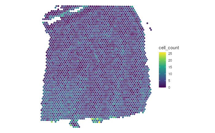

It is okay to use any combination of the add_* functions. For example, we want to show the spatial domains of the samples as the ground of the figure and use symbols to denote if each spot is within the outline of the tissue slice. In this example, all plotted spots are in the outlines of the tissue slice and hence marked with dots.

(p2 <- p |>
   add_ground(var = "ground_truth")) # round layer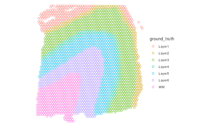

p2 |>
  add_symbol(var = "ground_truth", size = 0.2) # Symbol layer
#> Warning: The shape palette can deal with a maximum of 6 discrete values because more
#> than 6 becomes difficult to discriminate
#> ℹ you have requested 7 values. Consider specifying shapes manually if you need
#>   that many have them.
#> Warning: Removed 513 rows containing missing values (`geom_point()`).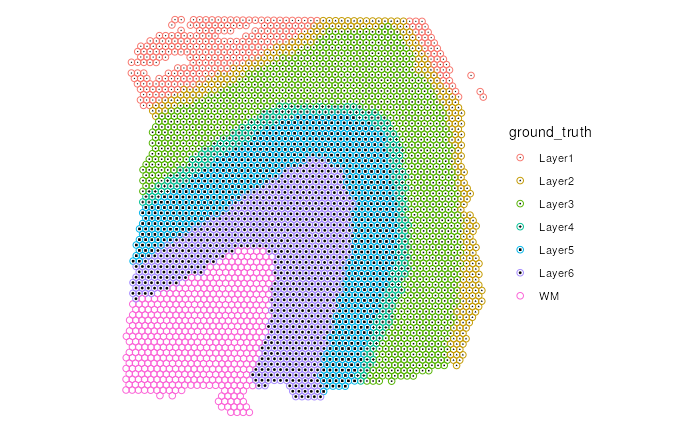

It is okay to change the ordering of these add_* functions. However, we advise to always have the add_fill as the first step to achieve the best visual effect due to the laying mechanism.

Customize escheR Plot

Choosing Color Palette for `add_fill` and `add_ground`

To maximize the utility of the multi-dimensional plot by applying both color-coded layers using add_fill() and add_ground(), it is important to choose minimally interfering color-palette for the fill and ground to avoid visualization confusion. The following demonstration provide some examples for simultaneously visualization of two variables regardless of their types (continuous vs categorical, or categorical vs categorical.)

Coninuous variable (gene expression) vs Categorical variable (Spatial Domains)

The following example visualizes the differential gene expression of MOBP, a marker gene for white matter, across different spatial domains. The default color palette, viridis, are not easily visible with color-coded spatial domains as there are overlapping in the color space, which could lead to possible confusion.

# Prep data
# Adding gene counts for MBP to the colData
spe$counts_MOBP <- counts(spe)[which(rowData(spe)$gene_name=="MOBP"),]

(p <- make_escheR(spe) |> 
    add_fill(var = "counts_MOBP") |> 
    add_ground(var = "ground_truth", stroke = 0.5))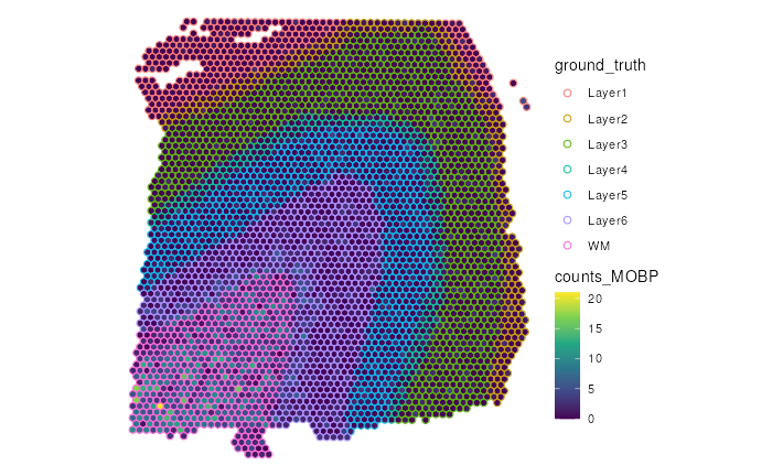

To improve the visualization, we choose to use a color that is not included in the color palette for ground_truth, which is the color black. Specifically, we use a color gradient from white (no expression) to black (maximum of gene counts) to represent the expression of MOBP in each spot. By using the white-black color gradient for the gene expression, we minimize the overlapping of the choice of color for spatial domains.

(p2 <- p + 
   scale_fill_gradient(low = "white", high = "black"))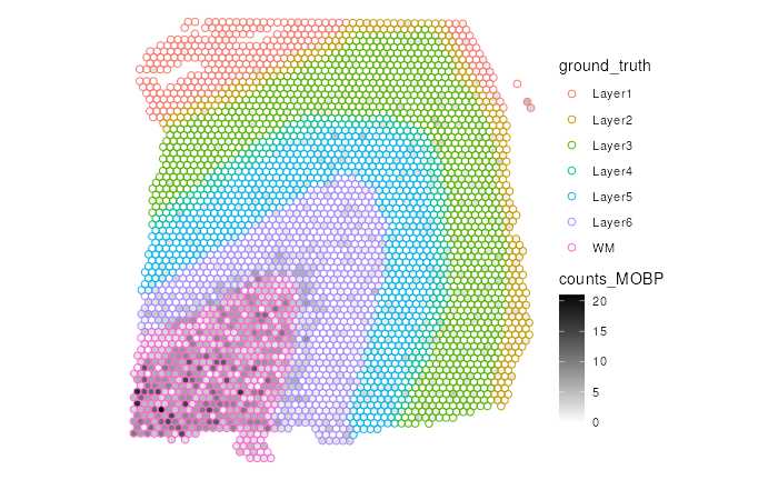

After customizing the color palettes to be minimally overlapping, it is easier to observe that MOBP has higher raw gene counts in the white matter (WM) region than other regions.

Categorical variable Vs Categorical variable

In this example, we demonstrate how to optimize color palettes for visualizing two categorical variables. We first create an arbitrary 5-level categorical variable called tmp_group, representing different horizontal regions of the tissue section.

spe$tmp_group <- cut(
  spe$array_row, 
  breaks = c(min(spe$array_row)-1 ,
             fivenum(spe$array_row))
)

table(spe$tmp_group)
#> 
#>  (-1,0]  (0,18] (18,36] (36,52] (52,73] 
#>      40     864     933     893     881

Following the principle to avoid overlapping of two color palettes, we use gradients of blue for different levels of tmp_group.

make_escheR(spe) |> 
  add_fill(var = "tmp_group") |> 
  add_ground(var = "ground_truth", stroke = 0.5) +
  scale_fill_brewer() +
  theme_void()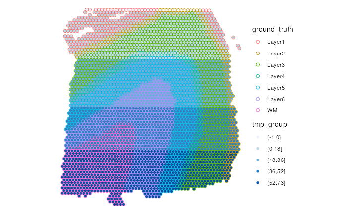

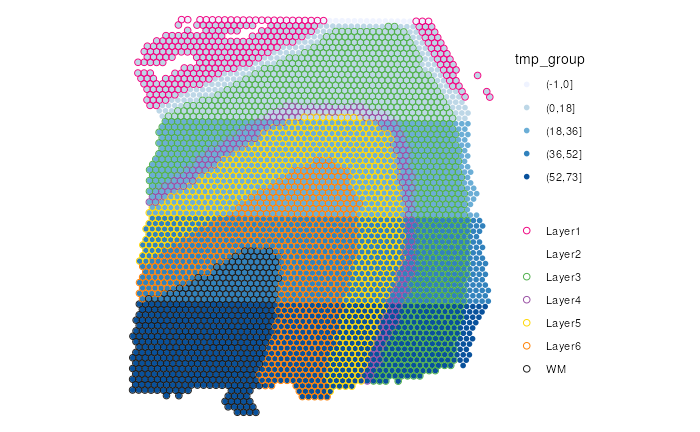
Here is another example where we try another manually-curated color-palette. We follow the same principle, minimize overlapping of two color-palettes for ground (scale_color_manual) and fill (scale_fill_brewer) respectively. Specifically, we use gradients of blue to show tmp_group and other colors for spatial domains ground_truth.

make_escheR(spe) |> 
  add_fill(var = "tmp_group") |> 
  add_ground(var = "ground_truth", stroke = 0.5) +
  scale_fill_brewer() +
  scale_color_manual(
    name = "", # turn off legend name for ground_truth
    values = c(
      "Layer1" = "#F0027F",
      "Layer2" = "transparent",
      "Layer3" = "#4DAF4A",
      "Layer4" = "#984EA3",
      "Layer5" = "#FFD700",
      "Layer6" = "#FF7F00",
      "WM" = "#1A1A1A")
  )

NOTE: It would be intrinsically difficult to construct a clear, intuitive and precise visualization when the number of categories/levels is large.

Guidance in choosing bivariate color palette

In this vignettes, we don’t provide or recommend specific color palettes, because the selection of color palettes is highly relevant to the underlying message and heterogeneous across analysis and studies, e.g. sequential palettes, qualitative palette, and divergent palette. Instead, we direct interested user to explore the topic on bivariate color palette. The blog post by Jakub Nowosad and R package biscale could be helpful to optimize your color palette for bivariate visualization.

In addition, if color palette is extremely to curate, e.g. large number of levels, it is possible to use symbols (add_symbol()) to annotate specific levels to avoid clutter in the color space.

Adjusting aesthetics

Given that the escheR package is developed based on ggplot2, aesthetics can be easily adjusted following the ggplot2 syntax. For example, given a escheR plot object, one can use + with theme_*, scale_* functions.

For example, to change the aesthetics of each layer, one can simply use the scale_* from ggplot2 to optimize the final visual presentation. For example, to optimize add_fill, one can use scale_fill_*; to optimize add_ground, one can use scale_color_*; to optimize add_sumbol, one use scale_shape_*. Here, we demonstrate how to change the color for the ground layer ( add_ground) using scale_color_manual.

(p_final <- p2 +
  scale_color_manual(
    name = "", # No legend name
    values = c(
      "Layer1" = "#F0027F",
      "Layer2" = "#377EB8",
      "Layer3" = "#4DAF4A",
      "Layer4" = "#984EA3",
      "Layer5" = "#FFD700",
      "Layer6" = "#FF7F00",
      "WM" = "#1A1A1A")
  ) +
  labs(title = "Example Title"))

Show a subset of levels

The easiest way to show only a subset of levels of a categorical variable is to create a new variable where all the unwanted levels will be set to NA values. Please see the example below

table(spe$ground_truth, useNA = "ifany")
#> 
#> Layer1 Layer2 Layer3 Layer4 Layer5 Layer6     WM 
#>    273    253    989    218    673    692    513

spe$tmp_fac <- factor(spe$ground_truth,
                      levels = c("Layer1", "Layer2"))
table(spe$tmp_fac, useNA = "ifany")
#> 
#> Layer1 Layer2   <NA> 
#>    273    253   3085

make_escheR(spe) |> 
  add_ground(var = "ground_truth") |> 
  add_symbol(var = "tmp_fac", size = 0.4) + 
  scale_shape_manual(
    values=c(3, 16),    #> Set different symbols for the 2 levels
    breaks = c("Layer1", "Layer2") #> Remove NA from legend
  )
#> Warning: Removed 3085 rows containing missing values (`geom_point()`).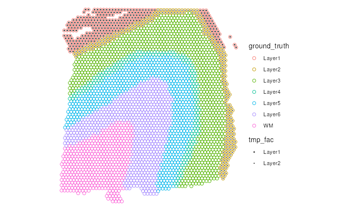

Multi-sample Figure

By design, make_escheR operates on only one sample. In order to create a figure compiling the spatial plots for multiple samples, individual plots are required via a series of calls to make_escheR, possibly via a for loop or an iterator function (e.g. lapply).

# Create a list of `escheR` plots
plot_list <- unique(spe$sample_id) |> # Create a list of sample names
  lapply(FUN = function(.sample_id){ # Iterate over all samples
    spe_single <- spe[, spe$sample_id == .sample_id]
    make_escheR(spe_single) |> 
      add_fill(var = "counts_MOBP") |> 
      add_ground(var = "ground_truth", stroke = 0.5))
# Customize theme
  })

Given all plots made for individual samples are stored in a preferred data structure (e.g. a list), one can use many functions, e.g. cowplot::plot_grid, patchwork, to compile and arrange individual plots to a paneled figure. The following example uses ggpubr::ggarrange to create a figure from a list of escheR plots.

library(ggpubr)
plot_list <- list(p2, p2)
ggarrange(
  plotlist = plot_list,
  ncol = 2, nrow = 1,
  common.legend = TRUE)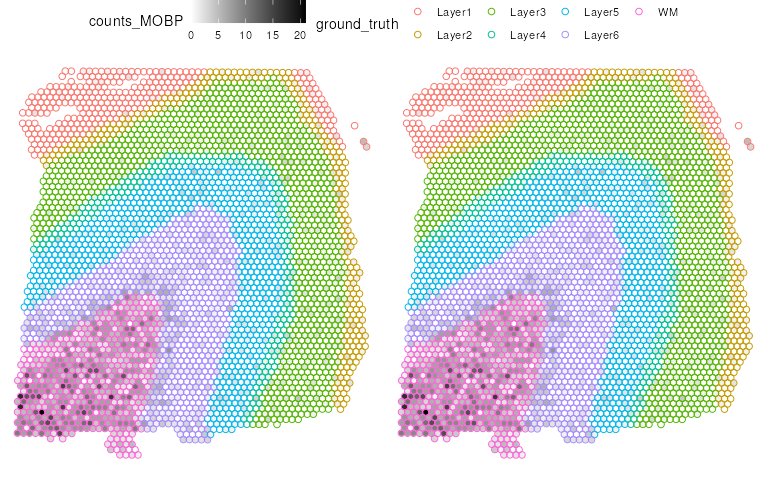

Save escheR plot

The procedure to save escheR plots is exactly the same as saving a ggplot object. In the example below, we use the function ggplot2::ggsave() to save escheR plots in the pdf format.

ggsave(
  filename = "path/file_name.pdf",
  plot = p_final
)

Session information

utils::sessionInfo()
#> R version 4.3.2 (2023-10-31)
#> Platform: x86_64-pc-linux-gnu (64-bit)
#> Running under: Ubuntu 22.04.3 LTS
#> 
#> Matrix products: default
#> BLAS:   /usr/lib/x86_64-linux-gnu/openblas-pthread/libblas.so.3 
#> LAPACK: /usr/lib/x86_64-linux-gnu/openblas-pthread/libopenblasp-r0.3.20.so;  LAPACK version 3.10.0
#> 
#> locale:
#>  [1] LC_CTYPE=en_US.UTF-8       LC_NUMERIC=C              
#>  [3] LC_TIME=en_US.UTF-8        LC_COLLATE=en_US.UTF-8    
#>  [5] LC_MONETARY=en_US.UTF-8    LC_MESSAGES=en_US.UTF-8   
#>  [7] LC_PAPER=en_US.UTF-8       LC_NAME=C                 
#>  [9] LC_ADDRESS=C               LC_TELEPHONE=C            
#> [11] LC_MEASUREMENT=en_US.UTF-8 LC_IDENTIFICATION=C       
#> 
#> time zone: UTC
#> tzcode source: system (glibc)
#> 
#> attached base packages:
#> [1] stats4    stats     graphics  grDevices utils     datasets  methods  
#> [8] base     
#> 
#> other attached packages:
#>  [1] ggpubr_0.6.0                STexampleData_1.10.0       
#>  [3] SpatialExperiment_1.12.0    SingleCellExperiment_1.24.0
#>  [5] SummarizedExperiment_1.32.0 Biobase_2.62.0             
#>  [7] GenomicRanges_1.54.1        GenomeInfoDb_1.38.5        
#>  [9] IRanges_2.36.0              S4Vectors_0.40.2           
#> [11] MatrixGenerics_1.14.0       matrixStats_1.2.0          
#> [13] ExperimentHub_2.10.0        AnnotationHub_3.10.0       
#> [15] BiocFileCache_2.10.1        dbplyr_2.4.0               
#> [17] BiocGenerics_0.48.1         escheR_1.3.2               
#> [19] ggplot2_3.4.4               BiocStyle_2.30.0           
#> 
#> loaded via a namespace (and not attached):
#>  [1] DBI_1.2.0                     bitops_1.0-7                 
#>  [3] gridExtra_2.3                 rlang_1.1.2                  
#>  [5] magrittr_2.0.3                compiler_4.3.2               
#>  [7] RSQLite_2.3.4                 png_0.1-8                    
#>  [9] systemfonts_1.0.5             vctrs_0.6.5                  
#> [11] stringr_1.5.1                 pkgconfig_2.0.3              
#> [13] crayon_1.5.2                  fastmap_1.1.1                
#> [15] backports_1.4.1               magick_2.8.2                 
#> [17] XVector_0.42.0                ellipsis_0.3.2               
#> [19] labeling_0.4.3                utf8_1.2.4                   
#> [21] promises_1.2.1                rmarkdown_2.25               
#> [23] ragg_1.2.7                    purrr_1.0.2                  
#> [25] bit_4.0.5                     xfun_0.41                    
#> [27] zlibbioc_1.48.0               cachem_1.0.8                 
#> [29] jsonlite_1.8.8                blob_1.2.4                   
#> [31] highr_0.10                    later_1.3.2                  
#> [33] DelayedArray_0.28.0           interactiveDisplayBase_1.40.0
#> [35] broom_1.0.5                   R6_2.5.1                     
#> [37] RColorBrewer_1.1-3            bslib_0.6.1                  
#> [39] stringi_1.8.3                 car_3.1-2                    
#> [41] jquerylib_0.1.4               Rcpp_1.0.11                  
#> [43] bookdown_0.37                 knitr_1.45                   
#> [45] httpuv_1.6.13                 Matrix_1.6-4                 
#> [47] tidyselect_1.2.0              abind_1.4-5                  
#> [49] yaml_2.3.8                    curl_5.2.0                   
#> [51] lattice_0.22-5                tibble_3.2.1                 
#> [53] shiny_1.8.0                   withr_2.5.2                  
#> [55] KEGGREST_1.42.0               evaluate_0.23                
#> [57] desc_1.4.3                    Biostrings_2.70.1            
#> [59] pillar_1.9.0                  BiocManager_1.30.22          
#> [61] filelock_1.0.3                carData_3.0-5                
#> [63] generics_0.1.3                RCurl_1.98-1.13              
#> [65] BiocVersion_3.18.1            munsell_0.5.0                
#> [67] scales_1.3.0                  xtable_1.8-4                 
#> [69] glue_1.6.2                    tools_4.3.2                  
#> [71] ggsignif_0.6.4                fs_1.6.3                     
#> [73] cowplot_1.1.2                 grid_4.3.2                   
#> [75] tidyr_1.3.0                   AnnotationDbi_1.64.1         
#> [77] colorspace_2.1-0              GenomeInfoDbData_1.2.11      
#> [79] cli_3.6.2                     rappdirs_0.3.3               
#> [81] textshaping_0.3.7             fansi_1.0.6                  
#> [83] S4Arrays_1.2.0                viridisLite_0.4.2            
#> [85] dplyr_1.1.4                   gtable_0.3.4                 
#> [87] rstatix_0.7.2                 sass_0.4.8                   
#> [89] digest_0.6.33                 SparseArray_1.2.3            
#> [91] rjson_0.2.21                  farver_2.1.1                 
#> [93] memoise_2.0.1                 htmltools_0.5.7              
#> [95] pkgdown_2.0.7                 lifecycle_1.0.4              
#> [97] httr_1.4.7                    mime_0.12                    
#> [99] bit64_4.0.5

Boyi Guo

Stephanie C. Hicks

Introduction

Installation

Input data format

Making escheR Plot

Load Packages

Preparing example data

Set up an `escheR` plot

Adding layers

Customize escheR Plot

Choosing Color Palette for `add_fill` and `add_ground`

Coninuous variable (gene expression) vs Categorical variable (Spatial Domains)

Categorical variable Vs Categorical variable

Guidance in choosing bivariate color palette

Adjusting aesthetics

Show a subset of levels

Multi-sample Figure

Save escheR plot

Session information

Getting Started with `escheR`

Boyi Guo

Stephanie C. Hicks

Introduction

Installation

Input data format

Making escheR Plot

Load Packages

Preparing example data

Set up an escheR plot

Adding layers

Customize escheR Plot

Choosing Color Palette for add_fill and add_ground

Coninuous variable (gene expression) vs Categorical variable (Spatial Domains)

Categorical variable Vs Categorical variable

Guidance in choosing bivariate color palette

Adjusting aesthetics

Show a subset of levels

Multi-sample Figure

Save escheR plot

Session information

Set up an `escheR` plot

Choosing Color Palette for `add_fill` and `add_ground`